


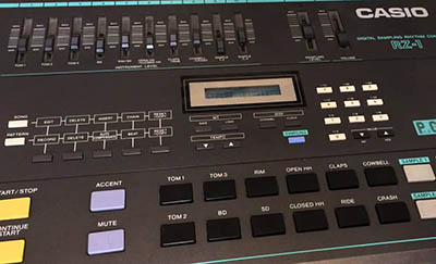
There are three ways to load samples into the Casio RZ-1: “cassette” dump via the MT (magnetic tape) terminal, MIDI SysEx, or in through the sample jack. The usual operating procedure is to sample through the mic/line-in jack for the initial sample creation and then export/import through the MT connection for archival/reload.
The MT port makes it possible not only to backup songs/patterns, but also to retain a perfect copy of whatever you’ve sampled into the Casio RZ-1. This capability not only retains sonic consistency of your samples, it also frees you from locating the original source material you sampled from each time you want to revisit a song.
At the time of the RZ-1’s release (1986) this was the only viable workflow as the RZ-1 unfortunately does not support MIDI SDS for sample dumps. But some 30 years later, another possibility appears: What if we convert a PCM wave file to the 8-bit / 20kHz format the RZ-1 needs and then load that sample via the MT import routine, thereby bypassing the RZ-1’s converters?
Note: Until recently, the ability for the RZ-1 to save/load via SysEx was almost entirely unknown. This feature has now been exploited much in the same way as the MT jack, but is still not equivalent to true MIDI SDS. However, it is much quicker and has effectively superseded the MT jack method described in this article.
Even if one prefers to utilize the analog sample input to add character, the MT import technique opens up the door for such things as tightening the attack (removing silence at the start of the sample), click removal, and mix-and-match loading.
Note: Due to its automatic transient detection method of sampling, the RZ-1 tends to leave about 0.013s of space in front of whatever is being input which leads to sloppy timing. DC offset, hum, and asymmetrical waveforms are other sampling anomalies that may occur.
Most RZ-1 users probably neglect to use the MT input/output jack as it’s not particularly well documented and the port uses an unusual and fairly non-standard wiring scheme of an 8-pin DIN (not to be confused with 5-pin MIDI).
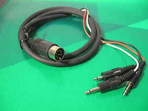
Fortunately, (aside from finding a full-sized 8-pin DIN connector) this cable is really simple to rig up. Advice for doing so is available on tinyloops.com. It’s for a different Casio device, but the principle remains the same. A few other music devices like the Yamaha DX11 use the same style connector for their cassette interfacing.
If you want the actual schematics for the Casio RZ-1, see below.
If you’re looking to purchase a ready-made cable for the RZ1, be prepared for a bit of searching; an MSX computer cassette cable is probably the best bet. They’re a bit hard-to-find, but can definitely be had for a manageable price with a bit of patience.
That solves our physical connection issues and lets us use the MT load/save feature as intended, but we still can’t import samples at will. To get this done, we need to figure out out two things: 1) The communication scheme/encoding of the MT port, and 2) Casio’s sample data format.
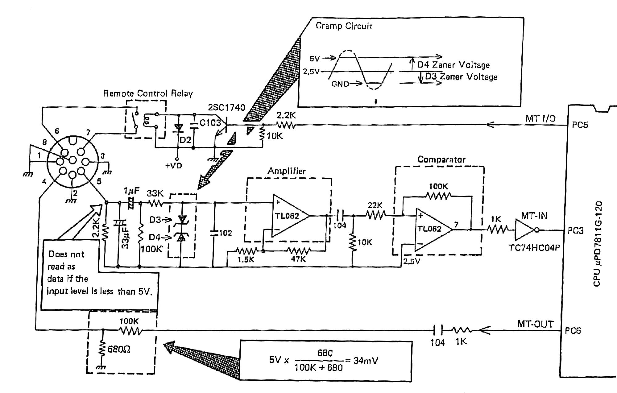
The service manual gives us a couple clues as to how the MT port communication scheme works:
Digital data of 1 and 0 are recorded on magnetic tape as 2.4KHz and 1.2KHz sound, respectively. When data is read, a signal from a cassette tape player comes in from MT terminal pin 5. Since the voltage level varies depending on cassette tape players, the two zener diodes cramp the signal between 0 and +5 volts.
The cramped waveform is amplified by the first opamp. The second stage opamp is a comparator which examines whether the input voltage is higher or lower than 2.5V and outputs a square waveform to CPU’s PC3 terminal.
As 5 volts of CPU’s PC6 terminal is too high for a cassette tape recorder, it is dropped to 34 millivolts by the 100Kohm and 680 ohm resistors.
Signal PC5 from MAIN CPU turns the remote control relay on and off which controls the motor in a cassette tape player.
The first paragraph is what we were looking for. This describes frequency-shift keying, which (not coincidentally) is a way that some vintage computers stored data to cassette. The MSX-style cable is another indicator of that methodology, as FSK is the exact same way the MSX computer talks to/from cassette tape.
There are many variants of FSK, so we’ve got to narrow it down a bit more to be useful. Using some common-sense and guesswork, the Kansas City Standard / Computer Users Tape Standard (CUTS) seems like a good starting point for investigating the RZ-1. The 1.2kHz/2.4kHz tone choice by Casio definitely fits with this, and the Casio TA-1 (rare as unicorn horns) documentation appears to be almost definitive proof (alert: red herring). One significant remaining question is its baud rate. If Casio was basing its designs off the MSX then 1200 baud would make sense, as that’s the rate supported by the MSX @ 1.2kHz/2.4kHz (1200 Hz/2400 Hz).
Here’s the gist of how 300 baud FSK works:
Data is coded as audio tones on the tape. A logic 0 consists of 4 cycles of a 1.2kHz tone, and a logic 1 consists of 8 cycles of a 2.4kHz tone.
Each byte (8 bits, LSB first) of data is preceded by a logic 0 start bit, and is terminated by a logic 1 stop bit. There is an additional parity bit before the stop bit. Each bit lasts for 3.33ms, giving a data transfer speed of 300 bits per second.
A recording is started with a lead-in of the 2.4kHz tone followed by the actual data.
1200 baud is the same except the amount of cycles are reduced to a quarter; a 0 bit is a single cycle 1.2kHz tone and a 1 bit is two cycles of a 2.4kHz tone. So let’s load our FSK dump into a wave editor and see what we’ve got.
At about the midpoint of the file, keep zooming until you can see the individual waveforms. There should be two distinct kinds which alternate back-and-forth, one narrower and one wider. The wide one is 1.2kHz and the narrower is 2.4kHz. To follow Kansas City Standard, the narrow waves should always be grouped evenly, but if they’re never in groups less than a multiple of 8 then we know we’ve got a 300 baud signal. If you can find narrow waves as a single pair then we’re at 1200 baud. Well… looks like we’re a bit off the mark because a couple things don’t match up.
Problem 1: We can see single cycles of 2400 Hz waves. This doesn’t fit in with any encoding schemes we’ve investigated so far, but the service manual does specify single cycle square waves of 2.4 kHz and 1.2 kHz, if read literally.
Problem 2: If we ignore the 2400 Hz leader tone at the start of our MT audio file (which is just a calibration tone and contains no data) and measure the time from the first 1200 Hz tone (the first 0 bit) until the end of the audio then we get something in the ballpark of 70-85 seconds depending on what is stored in the RZ-1. The time is fluctuating. How strange.
But problem 2 can tell us what our baud rate is supposed to be. Since the RZ-1 stores its custom sample data in two 64 kilobit chips (128 KBits total) then we should be expecting our MT data to translate to about 16 kilobytes of binary data (computer math for the win!) In other words, we need a 16,384 byte file to hold all the custom sample data on the RZ-1 which means we need at least 131,072 bits of communications data.
If we need to send 131,072 bits and only have approximately 70 seconds to transmit, then we need a data rate higher than 1200 baud, right? Even without the overhead of start/stop/parity bits we’d need at least 1800 bps.
The odd thing about this method is that 0 and 1 take different amounts of time to send. 0 takes twice as long as 1 because it’s half the frequency. In other words, transmitting a binary file of all 0s will take (ignoring the leader tone and any start bits, etc.) about 200% longer than a file that’s all 1s. If we make an MT dump of totally empty sample banks and compare its length to an MT dump containing sampled data then we will see that this is truly the case. So we’ve now determined that the average rate is around 1800 baud when the data is a 50/50 split between 1s and 0s, and it either exceeds or undershoots this rate depending upon the specific data being transferred.
That’s a pretty big diversion from the standards we’ve been considering. While sharing some of the same principles as the Kansas City standard, what we’ve deduced so far appears closer to the Sinclair ZX Spectrum / Amstrad CPC style cassette scheme which uses single pulses of square waves of two different widths, the natural result of which is a protocol that has a varying bit rate. Now we’re in the ballpark.
If we do a little more digging into specific obsolete tape storage methods, it appears the Tandy/Radio Shack cassette is a very close cousin to our mysterious Casio MT port. The TRS-80 series (CoCo, Model III, et al.) uses a 1800 averaging baud (1500 average bps), 2400/1200 Hz single-cycle square wave format. Bingo! We now know enough to convert the FSK data to a raw serial bit stream. In other words, we can take the beeps and boops and convert them to actual bits in a binary file to poke and prod. In fact, a TRS-80 program WAV2CAS by Knut Roll-Lind generates the raw bitstream more or less correctly, but we still need to convert the Casio bitstream into usable bytes before we can do anything productive with the data.
WAV2CAS adds an assumed 128 byte leader consisting of $55 bytes. We can safely strip that. We also need to strip the 7.99s calibration tone. We can do that by removing every 1 bit until reaching the first 0 bit.
Now we’re synchronized to the starting point of the serial data and can start figuring out how Casio encoded it.
The first thing we encounter in the bit stream is a similarity to the Model III and Atari cassette format which is a leader of alternating 1s and 0s, which in the MT signal is directly after the 7.99s long 2.4kHz calibration tone. In the Casio, this consists of a 0.03s burst of 42 alternating bits, directly followed with another 0.02s burst of 2.4 kHz tone. This could very well be designed to train for tape speed variance (speed measurement bits), but it’s very likely not important as data.
It’s fairly certain that the meaningful data starts directly after this, probably in some kind of “data block” and probably with some short identifying header or preamble. It’s hard to say exactly what that’s going to consist of, so let’s look for obvious patterns that jump out.
One of the most conspicuous is a reoccurring pattern of 111111110 which supports the (somewhat unusual) idea of a 9 bit byte. Stripping the last 0 gives us data bits of 11111111 which is 255 in decimal (FF in hex) which is the highest value possible. Likewise, 00000000 would be notable because it’s equal to 0 in decimal which is the lowest value possible. One of those two extremes are likely to be the most common values in a data file containing any amount of null space, such as audio silence or empty patterns.
It would seem obvious that we need to ditch the 0 to get our normal byte back, but let’s try to determine what it is and isn’t before charging forward with this assumption. The trailing 9th bit can’t be a stop bit because there would first need to be a start bit. That would extend us to 10-bit bytes (not likely for a variety of reasons), so let’s nix that idea. Instead of a trailing bit, it might actually be a start bit for the next set of bits, only with a stop bit omitted. Okay, let’s see if that theory holds up. A start bit would have to always be 0 in this case. If we can find strings of 1 that are longer than eight bits then that wouldn’t make sense because a start bit of 0 would prohibit this. Well, depending on where you look in the bit stream this idea might hold up, but given enough data points we can see that sometimes we get strings of 1 that exceed eight bits.
The only sane (read: traditional) possibility left is that the 9th bit is a parity bit. Find a section containing a clear 111111110 pattern and work left starting from the 0. The eight bits to the left of the 0 are composed of an even number of 1s (eight, in this particular case) and this is still preserved when including our starting bit of 0. Continuing left to the next set of 9-bits and we have either a 1 or a 0. If there’s an odd number of 1s in the eight bits to the left of that 9th bit then the 9th bit should be 1 because that additional parity bit “rounds” out the 1s to an even number. In other words, tally all the 1s in an eight bit section. If it’s odd then tack on a parity bit of 1 as the next bit in line; if it’s even instead then do likewise with 0 (Ex: 11000001|1 or 01111011|0). This method results in creating a 9-bit byte from an 8-bit byte which is exactly inline with our expectations.
Note: This scheme is known as ‘even’ parity. There is also ‘odd’ parity which results in the opposite value for the parity bit (Ex: 01111101|1 or 10001000|1). Any mention of parity with the Casio RZ-1 can be assumed to be of the even variety.
Keep following a known pattern of 111111110 backward long enough and you’ll hit other data that’s not so discernible. If the data isn’t corrupt then it should be consistent with our parity rules–and for the most part, it is. It’s clear that significant portions of data are in 9-bit format and only need the last 9th bit stripped to form a traditional 8-bit byte. But, just because the ghost of Casio past wants to make our lives a living hell, we can find sections which break this pattern. Meaning? We can’t proceed blindly in just stripping the parity bits to recover our data.
How are we going to reverse engineer ourselves out of this mess???!?! The anguish!!!
There are numerous other patterns we can discern if we probe more deeply, but let’s consider how to tackle this more elegantly:
The fortunate thing about the RZ-1 MT tape out procedure is that it’s divided into RHYTHM and SAMPLE. We obviously want to be working with the SAMPLE MT dump here as our goal is sample editing/replacement. While editing sequence/song data on the computer could be another interesting project, for our purposes we can ignore the RHYTHM dump feature. We know all four custom samples will be contained in any dump generated by the MT SAVE SAMPLE DATA routine, and we can also assume they’ll be in 20 kHz, 8-bit raw PCM as that’s what the RZ-1 uses internally (if you have an EPROM programmer you can actually replace the stock sounds in the RZ-1 via similar methods).
Let’s do some math to help us out.
Since we’re looking for chunks of PCM sample data, consider that it would make sense for each sample pad to be 32 kilobits (32,768 bits), since that’s 1/4 of the sample RAM available. With a sample rate of 20,000 Hz multiplied by a bit-depth of 8 we get 160,000 bps of PCM data. Divide the amount of bits available in RAM for each sample pad (32,768 bits) by our PCM data rate (160,000 bits per second) and we’ll get our amount of sample time per pad which is 0.2048s per pad = 0.8192s total. Okay, that all checks out with reality, so we’re on the right track.
Using some more math, we can figure out the parity bit overhead for a chunk of 32 kilobits. 32,768 bits divided by 8-bits per byte = 4096 bytes. Since each byte has one parity bit then our parity bit overhead is 4096 as well which makes the total number of bits per each sample pad (assuming no additional overhead) 36,864 bits.
Let’s look for chunks of around 36,864 bits that are suspicious.
Depending on what we’ve got sampled into the RZ-1, it is (or can be) evident that each sample pad is divided into 32 data blocks of 130 9-bit bytes each. When converted into traditional octet bytes, it is clear this is 2 bytes too many. We should have 128 data blocks with 128 bytes per data block for a total of 16,384 octets. Given that the RZ-1 has a verify feature when loading MT data, these 2 “extra” bytes are likely a checksum or CRC.
We can also notice that a pair of ’01’ bits is tacked onto the very end of each data block. This could be either a delimiter or simply padding to keep things lined up well for the 9/8 bits per byte difference, but they should be safe to ignore as actual data.
Once we convert the bitstream to usable bytes, we’ll be able to load the file into an appropriate application such as a wave editor or DAW.
So we just snap our fingers and convert the bitstream into octets, right? Wrong!!
Important things to know:
— The MT serial bitstream contains a header signifying whether it holds RHYTHM or SAMPLE data.
— Every 9th serial bit is a parity bit, but only in the general context of data blocks, not as a rule.
— Data blocks are terminated by a (non-data) delimiter.
— There are two extra (non-PCM) bytes per data block. One of these is an 8-bit modulo 256 checksum.
— The RZ-1 MT dumps are lsbit (least significant bit) first while signed 8-bit PCM 20,000 Hz data needs to be most significant bit first.
— Signed PCM data also utilizes a Two’s complement system where 00000000 is equal to 0 and 11111111 is equal to -1. In this system, a value of zero is considered a positive number.
— XORing each bit by 1 will toggle its value to the opposite (I.E. one becomes zero, zero becomes one).
Hint: From an engineering perspective, if a bit of 1 transfers twice as fast as a bit of 0 (2.4 kHz vs. 1.2 kHz) and we know that a large portion of our data is likely to be blank data then sending blank data as streams of 1s could cut average transmission time significantly.
Sounds like we’re going to have to code a custom application to decode the bitstream.
Note: See the link at the bottom of the page download the decoder.
So now that we’ve extracted our byte data from the serial bitstream, let’s load the binary we created from the MT dump into Audacity or Sound Forge as raw PCM data with the following settings: signed 8-bit, 20 kHz, mono.
Tech note: Since we’re working with only 8-bits (one byte) the endianness is irrelevant. LSbit vs. MSbit is a separate issue and needs to be addressed before this step.
If you now have a 0.82s file with 4 samples aligned at 0, 0.205, 0.410, and 0.615s then you’ve got it made. All we have to do is replace our samples with whatever we want, being careful to only overwrite the corresponding sample portion of the file, and at the correct alignments (given above). Remember that each sample is only 0.205s long.
For best results you’ll probably want to sample rate convert your samples from 44.1kHz (or 48/96/192) to 20 kHz with SoX, R8brain, or iZotope and bit-reduce from 16/24-bit to 8-bit with Waves L1 or similar.
After making your edits, save the file as a raw PCM of the exact same type. We don’t want any extra header info tacked on because the RZ-1 won’t know what to do with that. Besides, WAV files typically do not support signed 8-bit.
The penultimate step is to take our raw PCM file and convert it back to a serial bitstream. This demands a reinsertion of parity bits, delimiters, headers, etc. in the expected order or else the RZ-1 will rightfully consider the data as corrupt (read: unintentionally altered).
Note: To do so requires a custom application to encode the PCM data to a Casio serial bitstream. This encoder is included in the bundle available below.
The last step is to convert the bitstream back to FSK audio using the utility Play CAS (again by Knut Roll-Lind) and then use the “MT LOAD SAMPLE DATA” feature on the RZ-1 while playing back our newly created cassette tape FSK file.
Direct load of PCM sample data. Boom.